Hyperthermic - thermal maps for gliders
Note: you can jump straight to the maps.
Flying gliders is a fascinating activity. It requires certain knowledge from the area of meteorology, good intuition, swift reflexes, careful planning, and a lot of practice. To quote the pilot and writer Janusz Meissner:
Flying gliders is not only a sport: it is an art that provides a lot of aesthetic experiences, and gives the pilot a lot more pleasure that powered flight. It is only soaring that is real flying, because it is based on the knowledge of the air.
Modern technology is a great help to the art of gliding. GPS-based flight computers, electronic variometers, the FLARM collision avoidance system, modern numerical weather forecast customized to gliding - just to name a few things that every glider pilot is well familiar with.
Certified GPS recorders changed the way gliding competitions are held. Prior to the introduction of FAI-certified flight recorders, the competing pilots had to take timestamped photographs of certain points along the racing route, and present the results to the competition judges. Nowadays this procedure is reduced to submitting a digitally signed .IGC file from the flight recorder after landing.
The data
Thanks to the ubiquity of gliding flight recorders we are now equipped with large amounts of gliding data in the form of publicly available .IGC flight records. There are numerous Internet sites hosting competitions data, the biggest of them being Soaring Spot and On-line contest. These two sites hold, respectively, about 137.000 and about 681.000 flight records just from the years 2003-2013. On-line contest (OLC), however, has a policy that puts a ten flight downloads a day limit on the user, making it hard to obtain a reasonable number of flight records. That is why as of today I have not used any data from OLC.
The average size of an IGC file is about 230 kiB, and the average duration of the recorded flight is about 3 hours 50 minutes, basing on the data I have collected. I have accessed 140.000 IGC records, out of which 138.700 got parsed successfully and passed basic quality criteria. This gave me a total of 30,3 GiB of data, and 535.300 flight hours.
Certainly a lot of interesting information can be extracted from this data. The goal I have set for myself was to generate heat maps - i.e. maps that could tell the pilot where he should expect stronger thermal updrafts.
Terrain influence
It is a known fact that the meteorological phenomena allowing us to soar in the troposphere without an engine are often dependent on the shape and the nature of the underlying terrain. For example, mountain lee waves are a direct consequence of the presence of the wind above a mountain range during a period of stable temperature gradient in the troposphere.
Similarly, it is known that the terrain influences thermals activity in the boundary layer[1][2]. The theoretical model TherMap[3] is a good example of a direct approach to constructing a map of places where the probability of finding a thermal is higher basing on the shape of the terrain. As shown by ParaglidingNet[4], the results of the theoretical model TherMap are coherent with information extracted from paragliding flight records.
Interesting plots
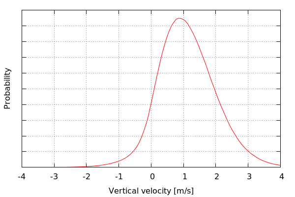
The general distribution of thermal's vertical velocity looks as follows (kernel density estimation with gaussian kernels). Suprisingly, the number of negative thermals, i.e. thermals in which the glider has lost altitude, is small, but not negligible.
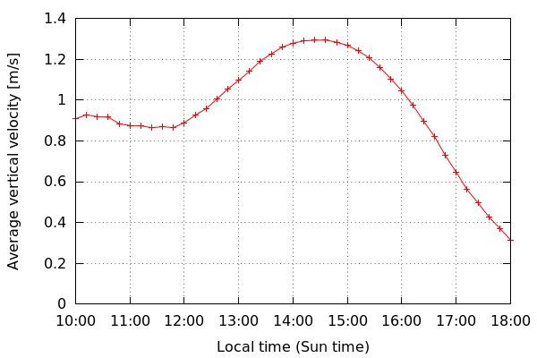
Vertical velocities averaged by local Sun time.
One can see that the best thermal conditions
kick in between 14:00 and 15:00 Sun time,
interestingly after 12:00, which is the hour
of the best radiation angle.
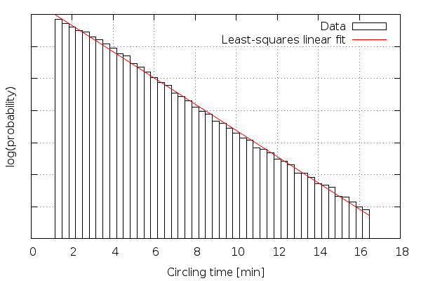
The following plot shows an unexpected property of
the data. The circling time - i.e. the time spent
inside a thermal - is exponentially distributed.
An interesting property of the exponential distribution
is that it is "past independent", which means that
during circling inside a thermal,
the remaining time that the pilot will spend in
a thermal is independed of the time he has already
spent. Or in other words: the decision about leaving
a thermal does not statistically depend on the time
the pilot has spent circling.
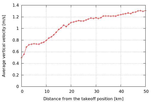
Plotting average thermal vertical velocity
versus the distance to the takeoff position
shows that there is a correlation between
these values. I attribute this property
mostly to the
fact that the vast majority of the data comes from
SoaringSpot, and therefore has been registered
during gliding competitions,
where the pilots don't have
an incentive to look for strong updrafts
before crossing the start line.
Because of that, for the purpose of map building,
I haven't used thermals that were
within the 20km radius from
the takeoff position.
The map problem
For the purpose of the map creation I will consider thermal to be a tuple of the following form: $$ T_i = \langle lat_i, lon_i, vv_i \rangle $$ where \(lat_i \in [-90^\circ, 90^\circ]\) and \(lon_i \in [-180^\circ, 180^\circ]\) are the WGS-84 coordinates of the thermal, and \(vv_i \in \mathbf{R}\) is the average vertical velocity of the thermal.
Map will be a function of the form: $$ M \colon [-90^\circ, 90^\circ] \times [-180^\circ, 180^\circ] \to \mathbf{R} $$ i.e. any function \(M\) that assigns vertical velocity to any point given its WGS-84 coordinates. The 2D plot of a fragment of the above function, along with basic geographic data, will be what people normally consider a map.
To evaluate the quality of a given map function \(M\) I've decided to use mean squared error (MSE), along with cross-validation, which is a common practice in machine learning. So, given a set \(\mathbf{T} = \{T_1, T_2, \ldots, T_n\}\) of thermals (data points) that were not used to create a map \(M\) I would estimate the performance of the map by computing the following metrics \(MSE_{rel}\): $$ MSE_{rel} = \frac{\sum_{i=1}^{n} (M(lat_i, lon_i) - vv_i)^2}{\sigma^2} $$ where \(\sigma^2\) is the biased variance estimator: $$ \sigma^2 = \frac{1}{n}\sum_{i=1}^{n}(vv_{avg} - vv_i)^2 $$ $$ vv_{avg} = \frac{1}{n}\sum_{i=1}^{n} vv_i $$
Maps
I have tested two approaches to the map problem, Hermite interpolation polynomials with linear least squares, and the k-nearest neighbors algorithm, with a custom weighted aggregation function, and haversine formula[5] as the distance function.
The k-NN algorightm delivered slightly better results in terms of cross-validated MSE, and much nicer looking maps. Through evaluation of the MSE metrics I've concluded that the optimal parameter k - the number of neighbors - should be equal to about 1000.
As a result I have generated the following maps:
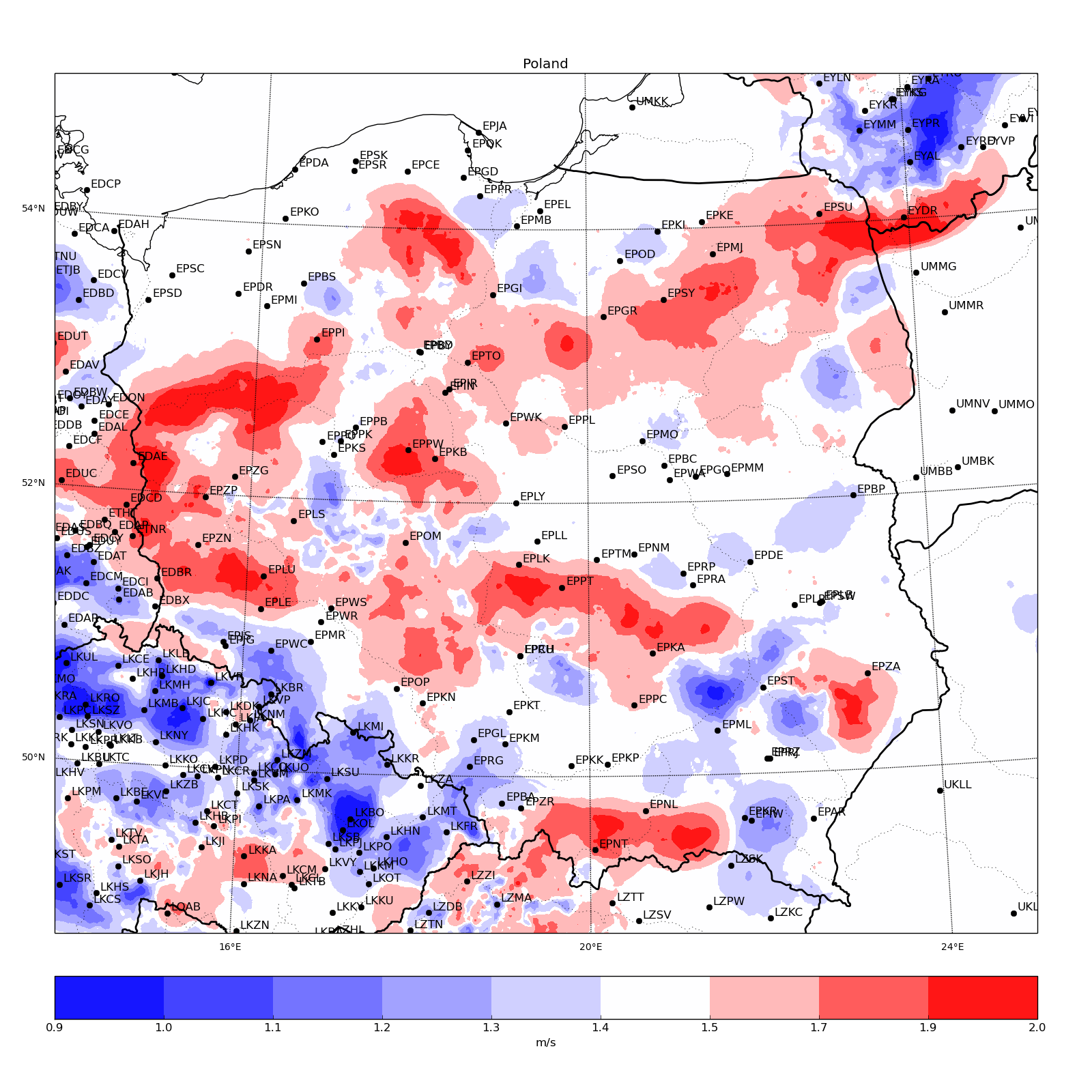
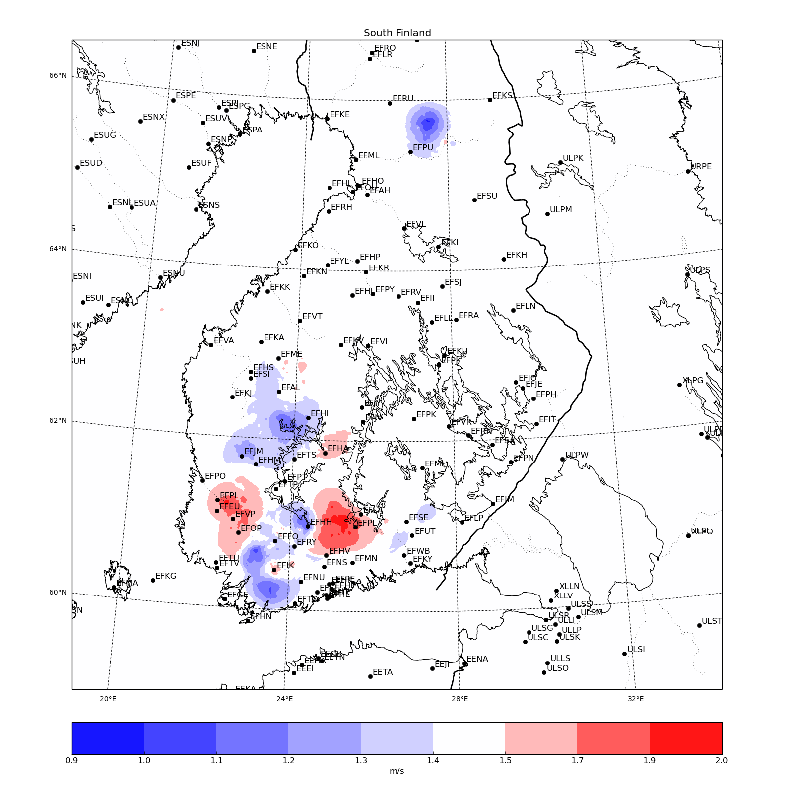
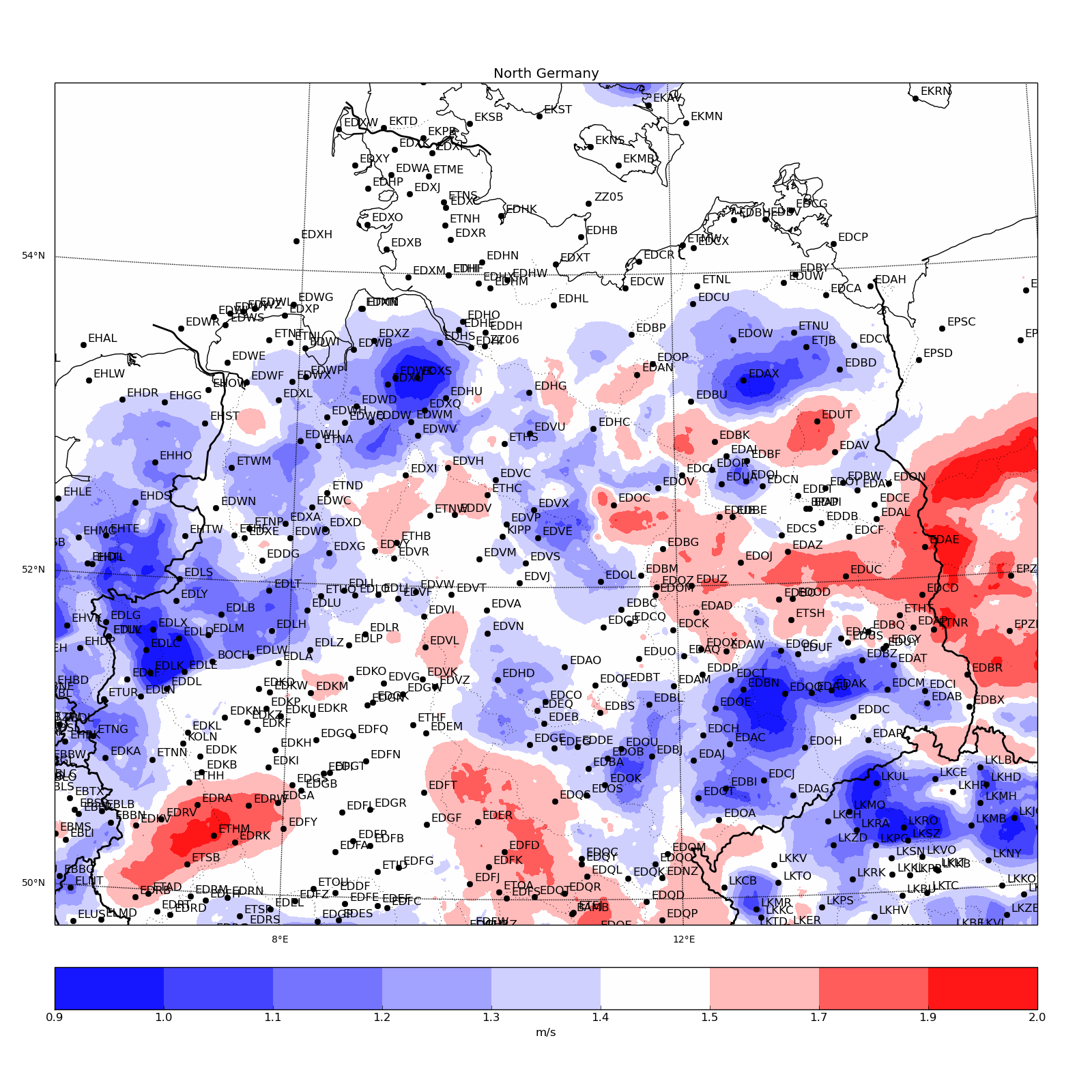
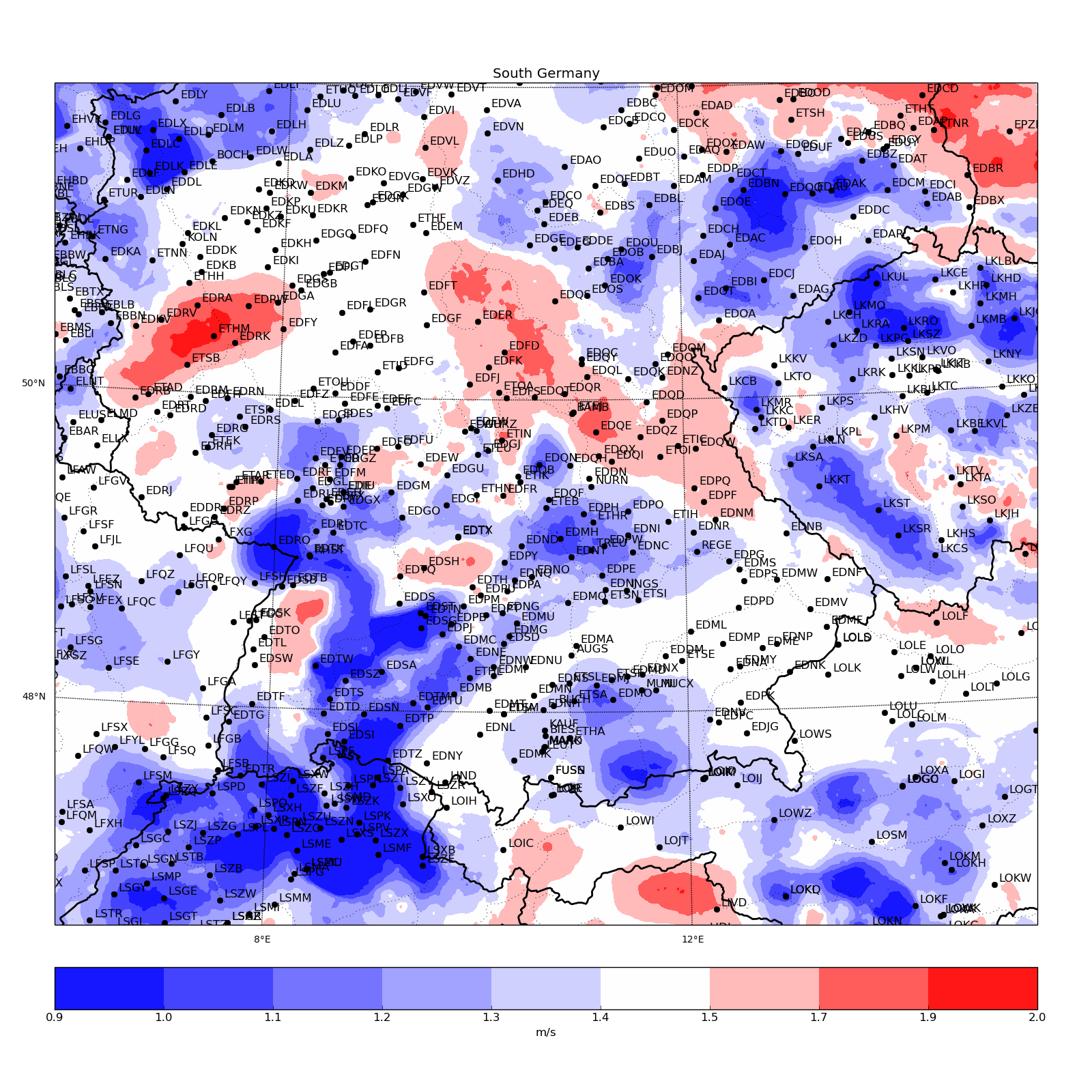
Future work
The prediction model I have presented estimates thermal's vertical velocity basing only on its location. It is very likely that more precision can be acheived by utilizing additional information, such as the time of the day (Sun radiation angle), the type of the glider (15 meter/open class, with/without water ballast), or the speed and the direction of the wind.
The paper
Hyperthermic was my bachelor's thesis at the University of Warsaw. You can download the thesis paper, it is in Polish only, sorry about that.
References
[1] Władysław Parczewski, "Meteorologia szybowcowa", Wydawnictwo Ligi Lotniczej, Warszawa 1953 (in Polish)
[2] Andrzej Abłamowicz, "Podręcznik pilota szybowcowego", rozdział 6, Wydawnictwa Komunikacji i Łączności, Warszawa 1967 (in Polish)
[3] Beda Sigrist, TherMap, http://www.aerodrome-gruyere.ch/thermap/
[4] Michael von Känel, ParaglidingNet, http://thermal.kk7.ch
[5] English Wikipedia, Haversine formula, http://en.wikipedia.org/wiki/Haversine_formula